Periodic Artifacts Generation and Suppression in X-ray Ptychography
by
 ,
,
Shilei Liu
1,2,3, 
Zijian Xu
1,2,4,*,
Zhenjiang Xing
5,
Xiangzhi Zhang
1,2,
Ruoru Li
1,2,3,
Zeping Qin
1,2,4,
Yong Wang
1,2 and
Renzhong Tai
1,2,4,* 1
Shanghai Synchrotron Radiation Facility, Shanghai Advanced Research Institute, Chinese Academy of Sciences, Shanghai 201204, China
2
Shanghai Institute of Applied Physics, Chinese Academy of Sciences, Shanghai 201800, China
3
School of Physical Science and Technology, Shanghai Tech University, Shanghai 201210, China
4
University of Chinese Academy of Sciences, Beijing 100049, China
5
Shenzhen Institute of Advanced Science Facilities, Shenzhen 518107, China
*
Authors to whom correspondence should be addressed.
Photonics 2023, 10(5), 532; https://doi.org/10.3390/photonics10050532
Submission received: 26 March 2023
/
Revised: 25 April 2023
/
Accepted: 30 April 2023
/
Published: 5 May 2023
(This article belongs to the Topic Advances in AI-Empowered Beamline Automation and Data Science in Advanced Photon Sources)
Abstract
:As a unique coherent diffraction imaging method, X-ray ptychography has an ultrahigh resolution of several nanometers for extended samples. However, ptychography is often degraded by various noises that are mixed with diffracted signals on the detector. Some of the noises can transform into periodic artifacts (PAs) in reconstructed images, which is a basic problem in raster-scan ptychography. Herein, we propose a novel periodic-artifact suppressing algorithm (PASA) and present a new understanding of PAs or raster-grid pathology generation mechanisms, which include static intensity (SI) as an important cause of PAs. The PASA employs a gradient descent scheme to iteratively separate the SI pattern from original datasets and a probe support constraint applied in the object update. Both simulative and experimental data reconstructions demonstrated the effectiveness of the new algorithm in suppressing PAs and improving ptychography resolution and indicated a better performance of the PASA method in PA removal compared to other mainstream algorithms. In the meantime, we provided a complete description of SI conception and its key role in PA generation. The present work enhances the feasibility of raster-scan ptychography and could inspire new thoughts for dealing with various noises in ptychography.
1. Introduction
Coherent diffraction imaging (CDI) has attracted extensive attention in the past decades. Since its first demonstration with X-ray by Miao in 1999 [1], numerous studies have been performed to improve this lensless imaging technique. Conventional lens imaging requires precise and high-cost focusing elements, and more significantly, its resolution is physically limited by the lens’s astigmatism. In contrast, CDI adopts an iterative phase retrieval algorithm to replace the imaging lens, and the object phase and/or amplitude can be reconstructed from diffracted patterns with an iterative algorithm. Its resolution is only limited by the light wavelength and the maximal diffraction angle available. X-ray ptychography, the most popular X-ray CDI method nowadays, combines CDI with sample scanning, thus generating a series of far-field diffracted patterns with high overlap (typically greater than 70%) between adjacent illuminated object areas by a localized probe, and the patterns are collected by a pixelated sensor, such as a charge-coupled device (CCD). Because of the high overlapping of the sampling areas, highly redundant diffractive information from the object and probe is acquired by the photosensitive sensor, which ensures highly efficient convergence of iterative reconstructions. On the other side, the scanning imaging method overcomes the object scale limitation of CDI, so that even a millimeter-scale specimen can be imaged with nanoscale resolution by ptychography [2].
However, various noises in experimental systems disturb ptychographic imaging, as in any other imaging method. Structured noise (such as parasitic scattering, ambient light, saturation, and dark noise), random noise (photon-counting noise, read-out, and detector noises), and outliers (bad frames, cosmic rays, and bad pixels) almost cover all kinds of possible noise and abnormal conditions [3]. Many advanced algorithmic innovations have frequently emerged in the past decade to overcome these noises and artifacts and enhance ptychographic imaging quality [4,5,6,7,8,9,10]. For example, the mixed-state method solves several decoherence problems related to the probe, sample, and detector, and the probe mixed-state technique has been a necessary optimizing tool in many new algorithmic developments [11]; position correction algorithms can retrieve the precise scan locations of the probe on the sample [12]; and the reciprocal-space up-sampling algorithm improves real-space resolution by fractionizing CCD pixels computationally [13]. In addition, an augmented projection method can correct position errors, rectify intensity fluctuations, and retrieve background noise with a rather complex mathematical formalism [14]. In recent years, artificial intelligence has been widely applied in nanometer imaging. The latest work attempted to solve the decoherent or pattern vibration problem by training a neural network based on DeblurGAN [15], which generates high-resolution diffracted patterns from low-resolution ones [16]. However, the ptychography reconstruction process is hard to completely replace by neural networks. In addition, recent works in EUV ptychography also provided valuable inspiration. These works include reconstructing periodic structures by applying vortex high harmonic beams [17,18], ultra-resolution EUV microscopy [19,20], applications of EUV coherent imaging in quantitative characterization [21,22], and so on.
Periodic artifacts (PAs), which are usually the result of the raster-scan scheme, can seriously degrade the quality of ptychography-reconstructed images, also known as the raster-grid pathology [23,24,25,26,27]. M. Dierolf et al. indicated that an unconstrained degree of freedom exists in the ptychographic phase of retrieval, which is relevant to the scaling ambiguity between the object and probe functions. When the scanning positions lie in a regular two-dimensional lattice (a raster-grid), this unconstrained degree of freedom will lead to the emergence of raster-grid pathology in the reconstructed image [28]. Therefore, the scaling ambiguity between the probe and object functions with a raster-scan grid is a key cause of the PAs. In addition to the raster-grid scan, other scanning schemes, such as circular scans or spiral scans, may also generate grid-like artifacts due to their local periodicity or approximate periodicity [29]. Compared to other scan schemes, the raster-grid scan is more likely to produce PAs. However, it is also one of the most important scan modes in scanning microscopy, as it is the easiest to implement and facilitates post-processing of image data in matrix form. Now, the raster-scan is still widely used in X-ray scanning imaging systems. In addition, through the raster-grid scan, ptychography is convenient to combine with other scanning imaging methods, such as scanning transmission X-ray microscopy (STXM) and X-ray fluorescence microscopy. Therefore, raster-scan ptychography has its unique advantages and should be retained as an important option in ptychographic imaging schemes.
Several approaches have been proposed to remove or suppress the grid pathology in raster-scan ptychography. One approach is to keep fixed certain known regions of the reconstructed object, such as a flat area or an artificial empty area, with only the diffraction of the probe alone being captured [28]. Breaking the symmetry of the scan grid is another important approach by using a non-periodic scan pattern [28,29]. Applying a probe support (mask) in reciprocal space during reconstruction is also an effective solution to suppress the PAs [30]. Based on previous ptychographic experiences, even weak noise in the high-frequency region of diffraction patterns can create obvious PAs in reconstruction results, as the high-frequency diffracted signals at the periphery of the CCD sensor decay so quickly that they are lower than noise.
In this article, we presented a concept termed static intensity (SI) that is another key generation cause of the PAs and proposed a novel periodic-artifact suppressing algorithm (PASA or PAS algorithm). The characteristics of SI are presented below:
- (1)
- No interaction with objects: The SI comes from the light or noise factors that do not interact with the object in the illuminated area, and it is incoherently added with the diffracted signals from the object and probe beam on the CCD plane.
- (2)
- Time invariability: The SI does not vary with time (scanning process), i.e., it is the static part in the recorded dataset and does not change with the scanned position of the object.
Therefore, each originally collected pattern contains the SI, while the SI may contain parasitic scattering from the upstream X-ray optical elements, ambient light scattered from the laser interferometer, thermal and readout noise of the detector, bad pixels and overexposure of the CCD, etc. These components also constitute the background noise, which should be the main part of the SI. Among these components, the X-ray parasitic scattering is produced together with the illuminating X-ray and cannot be captured by the CCD background measurement. The parasitic scattering may come from the stray light introduced by the X-ray elements, such as the order sorting aperture (OSA) [30], or from the high-order harmonic wave of the monochromator [31]. Both of the two parasitic scattering sources are considered incoherent signals to the illumination. Due to the inclusion of X-ray parasitic scattering, the SI cannot be removed by CCD background subtraction or by a calibration step in the experiment. It needs to be retrieved and separated during reconstruction.
We supposed that the SI is an important cause of PAs and is equivalently pivotal to grid pathology as the raster-scan grid. To separate SI from original collections and suppress grid pathology, we proposed the PAS algorithm, which includes an iterative update function for the SI and a binary circular support for the probe in the object plane. The SI update function was deduced through a gradient descent scheme for minimizing the cost function, as presented in Section 2. The robust ptychography imaging and grid artifact suppression performance of the PASA have been validated by both simulated and experimental data reconstructions in Section 3. A systematic comparison of the PASA method with state-of-the-art methods for suppressing grid pathology was conducted in Section 4, where the PASA showed unique advantages.
2. Periodic-Artifact Suppressing Algorithm (PASA)
The PAS algorithm was proposed based on a complete diffractive data model using a gradient descent scheme. In this model, a cost functional was constructed and differentiated to obtain the iterative update function of the SI, which was embedded in the extended ptychographic iterative engine (ePIE) [32] and used to iteratively separate the invariable intensity from multiple diffracted patterns. Additionally, a circular support for the probe in the object plane was applied in the object update function of the algorithm. This probe support constraint can effectively prevent the noise around the probe beam from entering the object function, somewhat similar to the OSA in the experiment.
As Figure 1 shows, a typical ptychography experimental facility (both for simulation and experiment) contained a zone plate (ZP) to focus the probe beam and an OSA to block secondary diffracted light downstream of the ZP. A specimen was placed downstream of the ZP focal point to have a larger illuminated area than the focus, and finally, a CCD detector was placed in the far field to record a series of diffracted patterns.
During measurement, a variety of noises are simultaneously captured by the CCD along with the diffracted signals. The noise changes with the object’s movement, so it can hardly be removed by directly subtracting background intensity from the data. Several approaches have been generally used to improve imaging quality in the presence of these noises [28,29,30]. On the experimental side, one can extend exposure time, increase the brightness of the probe beam to enhance the signal-to-noise ratio, or decrease the detector temperature to suppress the dark current noise. On the data-processing side, one can add a probe or object support to suppress the edge influence on reconstruction. However, these conventional solutions cannot completely remove the periodic artifacts (PAs) in ptychography. To deduce the PASA method and understand PAs more intuitively, we construct a complete ptychographic noisy data model, which shows how one diffracted pattern (Ii(q)) is collected during an exposure,
where and are the probe and object functions, respectively; is the displacement of the object from its initial location to the i-th illuminating point; and represent the vibration operators of the probe beam and object, respectively; and t is the illuminating time. It is assumed that within the exposure time interval, diffracted signals are accumulated linearly. Here, the static intensity is denoted by , which does not interact with the object and is scanning-position-independent, and is the weak random noise. We supposed that, in addition to the periodic scan grid or the scaling ambiguity between the object and probe functions, the SI is also a main generation cause of PAs because does not change with the object scanning, and for each scanned position on the object, the SI will leave some common signs or blurs after inversion of the diffraction pattern (containing the SI). These common signs over scanning positions will finally form the PAs on the reconstructed object and/or probe beam. Therefore, we concluded that, if the SI is removed from original data collections, the PAs in reconstructions can be mostly removed.
Herein, we mainly focused on PAs and their causes; thus, the vibration of the object and probe beam were both ignored, and the random noise was not explicitly considered, but it could be partially suppressed by the probe support constraint used in our new algorithm. Consequently, Equation (1) can be simplified as
To separate the SI from original datasets and suppress PAs in reconstructed images, we designed the periodic-artifact suppressing algorithm (PASA) based on the ePIE algorithm. In the PASA, we designed an additional iterative branch to update SI and incorporated probe support in the object update. The flowchart of the PASA is shown in Figure 2.
As the flowchart shows, the initial probe function and object function in real space are multiplied to generate the exit wave function on the object plane:
The diffractive wave field on the detector plane (phase space) is approximated as the Fourier transform of the exit wave from the object plane according to the far-field Fraunhofer diffraction theory:
To introduce the SI into the iterative reconstruction process, we designed a cost functional based on the least squares method. This functional contains the diffractive wave function of the i-th scanning point, the SI , and the original collection , and its formula is presented as:
which is also an error functional of the iterative reconstruction process. It can be simplified as follows:
where Ii(q) is the calculated total intensity on the reciprocal plane, as Equation (2) shows. By minimizing the functional by partially deriving it with respect to the modulus (square root) of the SI function and adapting it to the gradient descent form with a relaxation parameter [33], we obtained the iterative update function for SI:
In Equation (7), is always nonnegative. The iterative process of SI is shown in the flowchart in Figure 2 with thick arrows. The SI updating is performed at each scanning point of each iteration, which is the same as the probe update; therefore, the update parameter of SI, , is usually small. Here, we set to 0.3. The complete derivation process of the SI update function is shown in the Supplementary Material. According to our plentiful reconstruction experiences using the PASA, the final result is almost independent of the initial setting of . In our reconstructions, the initial was set as a random matrix ranging from 0.1 to 1.
After the SI is updated, the wave function in the detector plane is updated by replacing its amplitude with the measured and updating in the following manner:
Then, the exit wave in the object plane is updated by an inverse Fourier transform:
Similar to the ePIE algorithm, the object and probe functions are updated as follows, except for a support function acting on the probe in the object update:
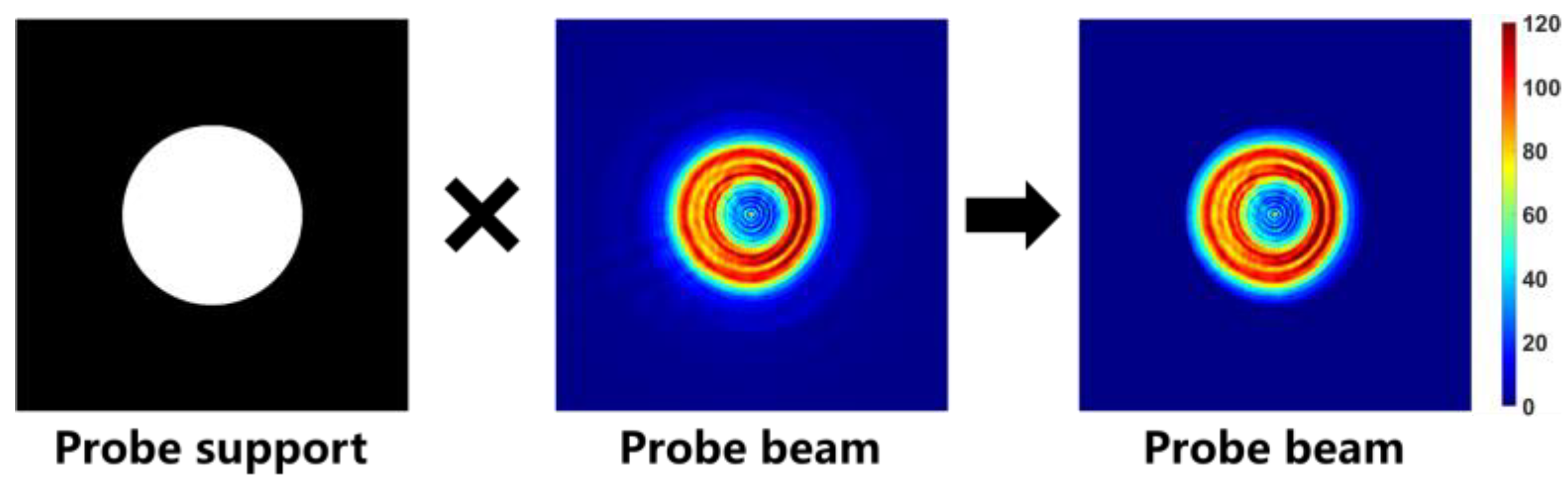
where is the binary support function to filter out the noise around the probe beam, as Figure 3 shows. Significantly, the support is only used in the object update (Equation (10)) but not in the probe update, similar to an aperture that only allows the probe beam to pass. This operation constrains the outer area of the probe function to block some random noise from hitting the object. The radius of the probe support is set to be a little larger than the probe radius to ensure the whole illumination beam can pass through. The above equations describe the calculation process for one scanning point of an iteration. As the iteration progresses, the SI is gradually separated from the datasets, and the remaining intensities will be relatively pure diffracted signals that will be reconstructed to clear object and probe images with no or fewer PAs.
3. Results
3.1. Parameter Settings
To investigate the cause of periodic artifacts (PAs) and verify the proposed PAS algorithm, both simulation and experimental data reconstructions were performed using the 1-probe-mode (1−PM) ePIE, 3-probe-mode (3−PM) ePIE, and 1−PM PAS algorithms for a systematic comparison. Moreover, the results using the PASA with or without the probe support were also given to show the effect of the probe support in suppressing the grid pathology. In addition, both the simulation and experiment share some common experimental settings, including the photon energy, the probe size, the scanning step size, and the zone plate (ZP) parameters, as shown in Table 1.
The experimental facility (both for the simulation and experiment, Figure 1) contained a ZP of 240 μm diameter with a 96 μm central stop and a 35 nm outermost zone width. A CCD detector was placed 60 mm downstream of the specimen. With a photon energy of 703 eV, the ZP can produce a focusing beam with NA = 0.0252. The specimen was placed 59.5 μm downstream of the ZP focus to obtain an illumination spot of 3 μm in size on the sample plane. In experimental data reconstructions, we used Fourier ring correlation (FRC) analysis [34,35] to assess the quality and resolution of reconstructed images. For both simulation and experiment reconstructions, the initial probe was constructed based on the Fresnel-Kirchhoff diffraction integral formula applied to the Fresnel ZP optics [36].
3.2. Simulation and Raster-Grid Pathology Cause Analysis
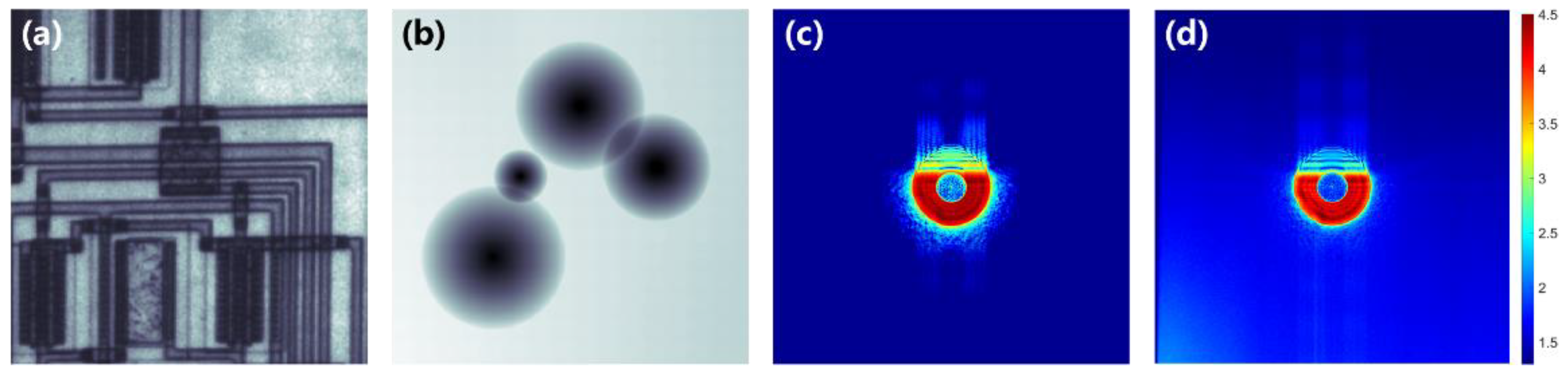
To verify the validity of the PASA and analyze the generation mechanism of PAs, several simulations were conducted with a realistic background distribution acquired at the BL08U1A beamline of the SSRF. In the simulated experimental setup, the detector was a CCD of 1024 × 1024 pixels with a 13 × 13 μm2 pixel size, and a 3-μm probe spot was used to scan the sample on a 15 × 15 raster-grid with a step size of 600 nm. For all simulations, an integrated circuit microscopic image (Figure 4a) and an image of several spheres with gradient intensities (Figure 4b) are used as the amplitude and phase-shift images of the simulative 2D complex sample, respectively. To simulate the real noise condition of ptychographic experiments, a series of real experimental background noise data were collected, averaged, and then added to the simulated diffractive signals, forming the main part of the SI. This background had gradient intensity values (brighter at the bottom-left corner, which may come from the ambient light scattered from the laser interferometer) and several bad lines. In addition, before being added to each pattern, this background noise was multiplied by a random fluctuating mask, whose values range from 0.95 to 1.05. The average intensity of the added background was around 1/100 of the centrally diffracted signals, and this signal-to-noise ratio was the same as that in the experiment data. Finally, each generated pattern was added to a 5% Gaussian-distributed noise to simulate the error of electronic signals. One generated diffracted pattern without (Figure 4c) and with (Figure 4d) noise is shown below.
To demonstrate the effect of a raster-scan grid on ptychography, random offsets of different magnitudes were added to the raster-grid scanning positions of the first simulations. Three comparative simulations with the maximal random offsets corresponding to 0%, 20%, and 40% step sizes (scanning grids were shown in Figure 5a–c), respectively, were performed using the 1−PM ePIE. The reconstructed amplitude results (Figure 5d–f) demonstrated that the PAs reduce as the random offset from the raster-grid rises. It is noteworthy that, in the 20% offset case, the PAs were still very protruding in the amplitude image, only a little weaker than those in the 0% offset result, indicating that an approximate periodicity in the scan grid can still lead to rather strong PAs. Nevertheless, obvious circular artifacts still existed in the 40% offset case, and the object details were not clearly reconstructed as well. In addition, the circles in the phase results can hardly be distinguished for all three offset cases. However, if no noise was added to the diffractive patterns, PAs would not exist in the reconstructed results, no matter if the raster-scan grid had any offset, as shown by the simulations in the Supplementary Material (Figure S1). This indicated that the raster-scan grid or the symmetric scanning position distribution is not the only cause of raster-grid pathology, and the SI (mainly made of background noise) contained in each diffraction pattern should also play a key role in the generation of PAs.
In experiments, the raster-grid scan without offset is widely used. Therefore, for the following simulations and experiments, we only adopted the regular raster-grid scan scheme.
As three kinds of noises were added to the simulated diffraction data, to distinguish the different effects of these noises (static background, fluctuating background, and Gaussian noise) on the PA generation, three additional simulations were performed using the ePIE algorithm with a raster-scan grid, and the results were shown in Figure S4 of the Supplementary Material. These results clearly demonstrated that either the background noise or the SI plays the key role in producing PAs, while the Gaussian random noise does not lead to PAs but rather random noise (blurring) and crosstalk between the amplitude and phase images.
In the subsequent simulations for validation of the PASA, three algorithms were used for comparison, including the 1−PM ePIE, 3−PM ePIE, and 1−PM PASA. In this case, the diffraction patterns contained strong SI, as shown in Figure 4d. Figure 6 shows the reconstruction results of these simulations. We can see that, as shown in Figure 6a,d, the 1−PM ePIE method could partially reconstruct the object structures and probe wavefront, but prominent PAs existed in both the amplitude and phase results, particularly the ring-shaped noises in the object image generated by the probe edge pseudo-intensity. These circles overlapped with each other and caused severe PAs. As for the 3−PM ePIE results (Figure 6b,e), the ring-shape artifacts were observably reduced, the details of the object became more distinct, and the form of the probe amplitude became more complete. However, periodic spot artifacts still remained in both the amplitude and phase images of the object and probe reconstructions. It could be inferred that increasing the probe mode number can promote reconstruction resolution, but it is far from enough to remove or suppress PAs in ptychography results. Finally, the PASA method was applied, and its results are shown in Figure 6c,f. We can see that the PAs were almost completely eliminated from both the amplitude and phase images of the object and probe reconstructions, with little random fluctuation remaining. The structure edges within the object were sharp and clear, and the reconstructed probe image was hardly contaminated by PAs. Therefore, the new PAS algorithm was validated by this simulation and proved to be much better than the multi-mode ePIE method in the presence of strong background noise (the main part of the SI).
During the PASA reconstruction, the SI was also recovered or separated from the diffraction patterns (Figure 7). Compared to the original added background noise (Figure 7a), the iteratively separated SI was almost the same as the original one. It can be seen that the distribution of the gradually varied background and even the bad lines on CCD were all successfully recovered. However, a bright annulus appeared in the center area of the recovered SI, yet it did not exist in the original one. This annulus was identified as a part of the SI, maybe because the intensity values in the central area are always the highest ones in each pattern, which contain some invariant components (such as the parasitic scattering from the upstream or over-exposure pixels) that would leave signs in the SI. Fortunately, this hardly influences the reconstruction results, as it is much lower than the central diffractive signals.
In addition, to demonstrate the effect of the probe support on PA suppression, we performed two simulations using the PASA without or with a probe support (Figure 8). One can see that slight periodic spot artifacts appeared in the result without any probe support (Figure 8a), while they were significantly suppressed in the result using a probe support in the object update (Figure 8b). We think that the PAs are mainly caused by the invariant and low-frequency noise in all diffracted patterns under the raster-scan condition, such as the gradually varied background shown in Figure 7a. The iterative process using the PASA would robustly separate the invariable SI from diffraction datasets, which carry the identical noise mode responding to different real space areas. The real-space noise corresponding to the invariable noise mode in the SI will accumulate in the overlapping areas of the adjacent illuminated points, and then the PAs are generated in reconstructed images. In a rigorous inspection, after the SI separation, slight fluctuations still exist as scanning progresses, forming weak periodic spots in the reconstructed result (Figure 8a, the red-boxed area), which are generally caused by the noise within the probe function window (for the Fourier transform) but away from the probe beam. While a probe support binary function was applied in the object update function (Equation (10)), these outer zone noises of the probe window were effectively filtered out (Figure 8c), hence the residual PAs were further suppressed (Figure 8b, especially the red-boxed area).
Without separation of the SI, the multi-mode probe method can only finitely improve the reconstruction results with a raster-scan grid (Figure 6b,e), probably because the SI mainly comes from the noise that does not interact with the object within the probe-illuminated area while all the probe modes of the multi-mode method interact with this object area; thus, the multi-mode ePIE cannot separate the SI as a probe mode and has little efficacy in suppressing PAs. PAs also appeared in the probe images reconstructed by the ePIE or multi-probe mode ePIE, as the object and probe functions are updated in a coupled way (Equations (10) and (11)), hence generating PAs simultaneously. On the contrary, the PASA provides an effective solution to PAs through the separation of the SI, which in turn provides a physical explanation for the PAs being generated. The above simulations preliminarily proved the feasibility of the PASA. Next, we would enter the experimental verification phase of the new algorithm.
3.3. Experiment
To further verify the effectiveness of the PAS algorithm and investigate its performance in the real world, a soft X-ray ptychography experiment dataset was reconstructed with the PASA. This dataset was collected at the Canadian Light Source (CLS) with a CCD detector of 1400 × 1400 pixels, with the pixel size being 13.5 μm × 13.5 μm. In this experiment, some Prussian-blue (ferric ferrocyanide) crystal particles were used as the specimen, and a 20 × 20 raster-grid was adopted for the ptychography scan, i.e., 400 diffractive patterns were collected. Similar to the simulations shown in Figure 6, no random position offset was added to the raster-grid. In addition, the CCD background noise was acquired without X-ray illumination before the sample measurement, and all the experiment diffraction patterns were subtracted by this CCD background before reconstructions. In this part, we adopted the same three algorithmic schemes as in the simulations to reconstruct the experiment data: the 1−PM ePIE, the 3−PM ePIE, and the 1−PM PASA. Each reconstruction was performed for 200 iterations, and the final results are shown in Figure 9. The FRC analysis, an acknowledged resolution estimation method, was used to quantitatively assess the reconstruction results and evaluate their resolutions.
As Figure 9a shows, obvious periodic artifacts (PAs) can be seen in the 1−PM ePIE result, although the background-subtracted SI was only about 1/100 of the illuminating intensity. One can see the sharpness of the object was quite poor, as indicated by the structure details within the red-box-framed region. When the 3−PM ePIE method was used, the PAs were still in the reconstructed image (Figure 9b), even becoming a little more prominent than those in the 1−PM ePIE result. It can be seen that evident meshes covered the whole object area, which lowered the visibility and authenticity of the object details, although the reconstructed structures became a little more distinct than those in the 1−PM ePIE result, as indicated by the red-framed area of Figure 9b. However, when the 1−PM PASA method was applied, as expected, great improvements in imaging quality could be seen in the reconstruction result (Figure 9c). Compared with the 3−PM ePIE and 1−PM ePIE results, not only did the PAs almost completely disappear in the PASA result, but also the sharpness and resolution of the reconstructed object details increased dramatically, as demonstrated in the red-boxed area. On the physical side, the PASA method successfully separated an SI from the original patterns (after subtraction of the CCD background), as shown in Figure 10, where one of the original patterns was iteratively separated into a clear diffractive pattern and the common SI for all patterns. The clear pattern had a clear background in the surrounding area while retaining high-definition diffracted signals in the central area. Consequently, a high-resolution object image would be obtained from these clear patterns. Significantly, two pretty strong concentric light rings appeared in the separated SI (Figure 10c), just around or within the central diffraction annulus. These two light rings, or halos, can be attributed to the X-ray parasitic scattering (stray light) that is introduced by the OSA and/or ZP edges. This kind of noise does not exist in the CCD background, which is collected without the probe beam illumination.
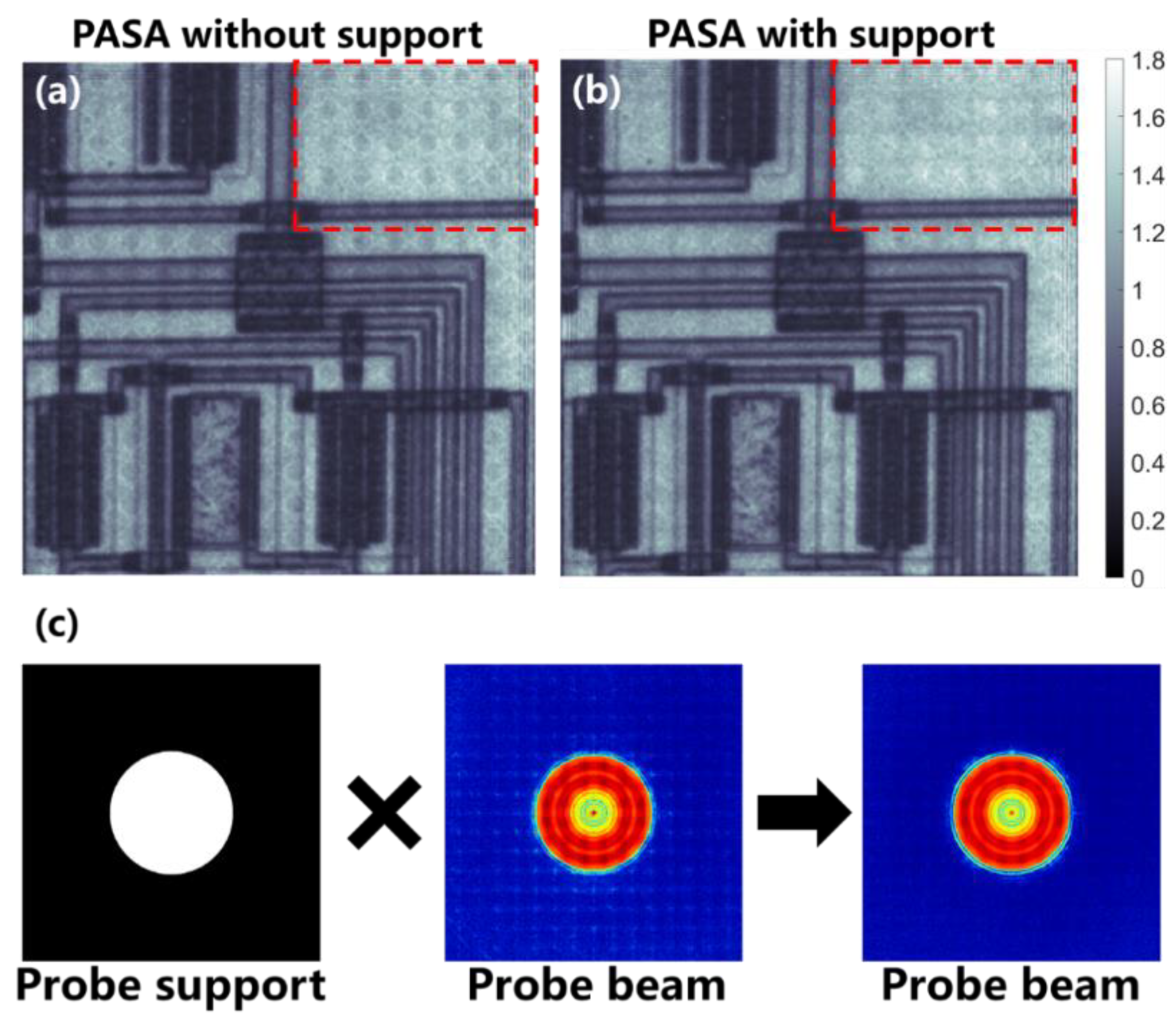
The effect of the probe support on PA suppression was demonstrated by comparing the two PASA reconstructed results with or without a probe support, as shown in Figure 11. One can see that the PASA without a probe support could not fully remove the periodic mesh-grid noise (left half image of Figure 11a). However, when a probe support was added to the object update of the PASA, the periodic noise was almost entirely removed (right half image of Figure 11a). The same conclusion can be derived from the reconstructed phase results in Figure 11b. An investigation of the influence of probe support radius on the PASA reconstruction was also performed, as shown in the second part of the Supplementary Material. The results (Figure S2) suggested that the probe support radius should be set to around 20–30% larger than the real probe radius so that the best PASA reconstruction result can be obtained.
Finally, a series of quantitative analyses, including the FRC analysis (Figure 12a) and the resolution-time mapping (Figure 12b), were performed on the reconstruction results to further confirm the advantage of the PASA method. For each of the three algorithmic schemes considered above, the result was obtained by averaging 10 repetitive reconstructions with different random initial functions to avoid accidental singular values. In the FRC analysis, we found that the spatial resolutions of the reconstructions by using the 1−PM ePIE, 3−PM ePIE, and 1−PM PASA methods were 35.33 nm, 19.28 nm, and 14.62 nm, respectively. In the resolution-time mapping analysis, it can be seen that the 1−PM PASA reconstruction took much less time than the 3−PM ePIE one but achieved a significantly higher resolution than the other two conventional methods, indicating an extraordinary high efficiency of the PASA method.
4. Discussion
The raster-grid pathology is a basic problem in ptychography with a raster-scan grid. In the methodology section, we proposed the concept of static intensity and assumed that, in addition to the raster-grid (the scaling ambiguity between the object and probe functions), the SI is also a key cause of periodic artifact (PA) generation. The physical definition of SI is the constant intensity part of diffractive patterns that does not change with the scanning of the object’s position in a ptychography experiment. For each scanned position on the object, the SI will leave some common signs after the inversion of the pattern. These common signs over scanning positions will form the PAs on the reconstructed object and/or probe beam. As the iteration progresses, the most overlapped spots will be the places where PAs are more prominent than elsewhere. Therefore, if the invariant SI is removed from the original patterns, the PAs can be mostly removed simultaneously. This is well demonstrated by the simulative and experimental data reconstructions using the proposed PASA method. It is worth mentioning that a previous work also considered a constant background noise over different diffraction patterns [14], which is similar to the conception of SI. However, that method is more complicated in math and needs more time to iteratively modify its shrinkage parameter. Moreover, that work did not investigate the effect of that method on grid pathology. In our work, we proposed a brief conception of SI that is dedicated to PA generation and suppression and the relevant PAS algorithm that is simple, efficient, and robust in iterative calculations.
Under real experimental conditions, many complex factors can affect imaging quality, including the ambient light leaked into the chamber, the upstream parasitic scattering, the scattered light from the laser interferometer, the thermal and readout noise of the detector, etc. These noise factors constitute the incoherent background noise on the CCD and also make up the main part of the SI. Among these components, the X-ray parasitic scattering is produced together with the illuminating X-ray and cannot be captured by the CCD background measurement. In the synchrotron radiation beamlines, this kind of scattering has been proven to be widespread. The parasitic scattering may come from two sources: one is the stray light introduced by the upstream X-ray elements, such as the OSA or ZP [30], and the other is the high-order harmonic wave from the beamline monochromator with a photon energy two or three times that of the illuminating X-ray [31]. In addition, the CCD saturation, bad pixels and bad lines are also common negative factors, which would enter the SI and bring more PAs into the results. All these noise factors can be effectively dealt with using the PASA method. In hard X-ray ptychography, the noise situation is somewhat different, as some of the noise sources (such as ambient light and readout noise) have little effect on the mainstream hard X-ray detectors. Therefore, the proposed method is more advantageous in the soft X-ray and visible light regimes than in the hard X-ray regime.
However, it was found that the SI separation operation could not thoroughly remove periodic noises, and weak periodic spots still exist in the reconstructed result. This may be due to the imperfect refinement of the SI during a limited number of iterations in reconstructions. These weak PAs are probably relevant to the noise within the probe function window but away from the probe beam (the noise in the probe beam scope has little effect as it is much lower than the central signals), and this noise should originate from the residual SI on the reciprocal plane. Hence, the addition of a probe support in the object update (Equation (10)) is a useful trick to filter out this noise (or residual SI) and further suppress residual PAs. In addition, a probe support in real space could prevent singular values from appearing in the object function.
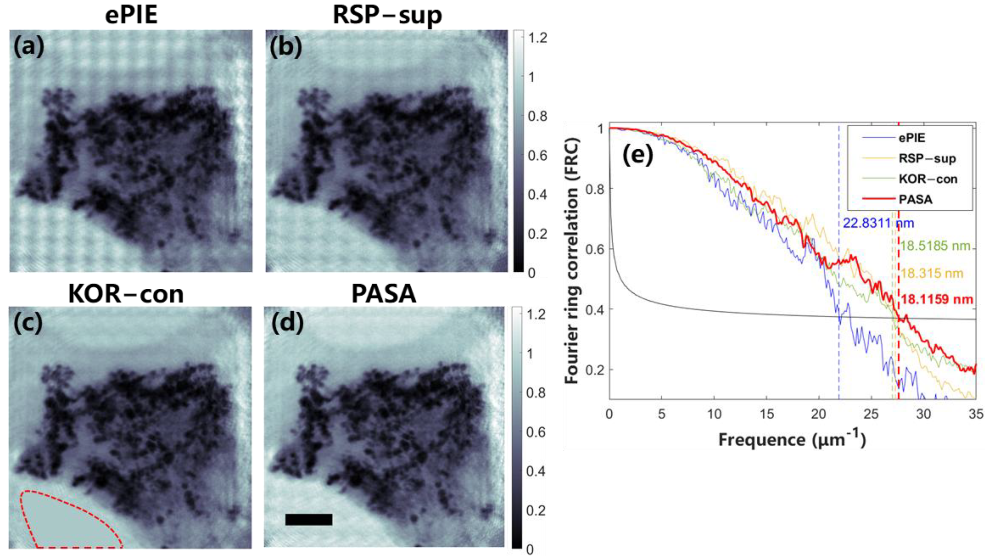
Several previous approaches for suppressing the grid pathology have been mentioned in the Section 1, including the known object regions constraint (KOR−con), the reciprocal space probe support (RSP−sup), etc. We compared two of them (KOR−con and RSP−sup) with the PASA and ePIE methods using a ptychographic dataset acquired at the BL08U1A beamline of SSRF. Herein, Pt-Co alloy nanoparticles on the carbon film of a copper grid were used as the specimen, and an 8 × 8 raster-grid with a maximal random offset of 20% step size was scanned. All reconstructions were performed using a 3−mode probe for 100 iterations, and the reconstructed amplitude results are shown in Figure 13. The reconstructed phase results and an STXM image of the specimen are shown in Figure S3 of the Supplementary Material.
As Figure 13a shows, strong PAs can be seen in the ePIE result, while Figure 13b shows that the PAs were effectively reduced by the RSP−sup method, although still visible. Figure 13c shows the KOR−con result with even weaker raster-grid pathology than that of the RSP−sup result, demonstrating that the KOR−con method has a higher ability to suppress PAs than the RSP−sup method. In this figure, the known region was circled by red-dashed curves, and it was a void area (fully transparent), which was kept constant during reconstruction. However, the KOR−con method requires that the specimen really has such a known flat region and its accurate location is known a priori, or an extra measurement of the probe diffraction pattern alone is performed to artificially create an additional empty object area. These a priori information requirements decrease the applicability of the KOR−con method. Finally, when the PASA method was used (Figure 13d), the PAs in the reconstructed object amplitude image were eliminated almost entirely, and a cleaner object image than the other three results was obtained without using any additional a priori information, demonstrating the unique advantage of the PASA method over the other three. The FRC resolution analysis (Figure 13e) further confirms the above conclusions from the observation of reconstructed images, as the resulting spatial resolution of the PASA reconstruction (18.12 nm) is higher than those of the ePIE, RSP−sup, and KOR−con reconstructions (18.32 nm, 18.52 nm, and 22.83 nm, respectively).
5. Conclusions
This work focused on periodic artifacts (PAs) or raster-grid pathology in ptychographic imaging with a raster-scan grid. We not only provided a new understanding of the PA generation mechanism, which includes the static intensity (SI) as an important cause of PAs, but also proposed a novel periodic-artifact suppressing algorithm (PASA), which combines the SI iterative separation with a probe support constraint embedded in the object update to remove this kind of noise. The proposed conception of SI in combination with the raster-grid (i.e., the scaling ambiguity between the object and probe functions) is the key to understanding how PAs are generated and how to remove them. Both simulated and experimental data reconstructions demonstrated that the new PASA method could almost completely separate the SI from the original datasets and greatly suppress the grid pathology, thus observably improving the resolution of reconstructed images with the purified diffracted signals. The PASA method showed better performance in suppressing PAs when compared to state-of-the-art algorithms. As a result, this new algorithm enhances the feasibility of ptychography imaging with a raster-scan grid.
The PASA method is applicable to most ptychographic cases, including 2D and 3D imaging methods such as ptychographic X-ray tomography [37], virtual depth-scan ptychography [38], position-guided vibration separation ptychography [39], etc. In the next step, we will generalize the algorithm to merge with other ptychography approaches to increase their applicability under the raster-scan condition. In addition, machine learning will be introduced into our following work to optimize the SI reconstruction with better robustness and deal with random noise modes and other factors that reduce ptychography quality by using deep neural networks. It is expected that random noise modes will become highlighted after the separation of SI by the PASA, and the further treatment of random noises by machine learning or other methods may be relatively easy without disturbing the static intensity.
Supplementary Materials
The following supporting information can be downloaded at: https://www.mdpi.com/article/10.3390/photonics10050532/s1, Figure S1: Do periodic artefacts (PAs) solely come from raster grid scan? Figure S2: The influence of probe support radius on PASA reconstruction; Figure S3: STXM and reconstructed phase images of the Pt-Co alloy nanoparticle sample; Derivation of the SI update function; Figure S4: Influence of different kinds of noises on generation and suppression of PAs.
Author Contributions
Conceptualization, S.L. and Z.X. (Zijian Xu); methodology, S.L., Z.X. (Zijian Xu) and Z.X. (Zhenjiang Xing); software, S.L., Z.X. (Zijian Xu) and Z.X. (Zhenjiang Xing); validation, Z.X. (Zijian Xu), Y.W. and X.Z.; formal analysis, S.L. and Z.X. (Zhenjiang Xing); investigation, S.L. and Z.X. (Zijian Xu); resources, Z.X. (Zijian Xu), Y.W. and R.T.; data curation, S.L., Z.X. (Zijian Xu), Z.X. (Zhenjiang Xing) and R.L.; writing—original draft preparation, S.L.; writing—review and editing, Z.X. (Zijian Xu); visualization, S.L. and Z.Q.; supervision, Z.X. (Zijian Xu) and R.T.; project administration, Z.X. (Zijian Xu) and R.T.; funding acquisition, Z.X. (Zijian Xu), Z.X. (Zhenjiang Xing), X.Z. and R.T. All authors have read and agreed to the published version of the manuscript.
Funding
This research was funded by Ministry of Science and Technology of the People’s Republic of China (2022YFA1603702, 2021YFA1601001); National Natural Science Foundation of China (11875316, 12175296, 12205206); Science and Technology Commission of Shanghai Municipality (21JC1405100).
Institutional Review Board Statement
Not applicable.
Informed Consent Statement
Not applicable.
Data Availability Statement
Data will be made available upon reasonable request.
Acknowledgments
Authors thank the BL08U1A beamline of Shanghai Synchrotron Radiation Facility (SSRF) and the SM beamline of Canadian Light Source (CLS) for providing beamtime.
Conflicts of Interest
The authors declare no conflict of interest.
References
- Miao, J.; Charalambous, P.; Kirz, J.; Sayre, D. Extending the methodology of X-ray crystallography to allow imaging of micrometre-sized non-crystalline specimens. Nature 1999, 400, 342–344. [Google Scholar] [CrossRef]
- Jiang, Y.; Deng, J.; Yao, Y.; Klug, J.A.; Mashrafi, S.; Roehrig, C.; Preissner, C.; Marin, F.S.; Cai, Z.; Lai, B. Achieving high spatial resolution in a large field-of-view using lensless X-ray imaging. Appl. Phys. Lett. 2021, 119, 124101. [Google Scholar] [CrossRef]
- Chang, H.; Enfedaque, P.; Zhang, J.; Reinhardt, J.; Enders, B.; Yu, Y.-S.; Shapiro, D.; Schroer, C.G.; Zeng, T.; Marchesini, S. Advanced denoising for X-ray ptychography. Opt. Express 2019, 27, 10395–10418. [Google Scholar] [CrossRef] [PubMed]
- Takahashi, Y.; Suzuki, A.; Zettsu, N.; Kohmura, Y.; Senba, Y.; Ohashi, H.; Yamauchi, K.; Ishikawa, T. Towards high-resolution ptychographic X-ray diffraction microscopy. Phys. Rev. B 2011, 83, 214109. [Google Scholar] [CrossRef]
- Maiden, A.; Humphry, M.; Sarahan, M.; Kraus, B.; Rodenburg, J. An annealing algorithm to correct positioning errors in ptychography. Ultramicroscopy 2012, 120, 64–72. [Google Scholar] [CrossRef] [PubMed]
- Edo, T.; Batey, D.; Maiden, A.; Rau, C.; Wagner, U.; Pešić, Z.; Waigh, T.; Rodenburg, J. Sampling in X-ray ptychography. Phys. Rev. A 2013, 87, 053850. [Google Scholar] [CrossRef]
- Beckers, M.; Senkbeil, T.; Gorniak, T.; Giewekemeyer, K.; Salditt, T.; Rosenhahn, A. Drift correction in ptychographic diffractive imaging. Ultramicroscopy 2013, 126, 44–47. [Google Scholar] [CrossRef]
- Pelz, P.M.; Guizar-Sicairos, M.; Thibault, P.; Johnson, I.; Holler, M.; Menzel, A. On-the-fly scans for X-ray ptychography. Appl. Phys. Lett. 2014, 105, 251101. [Google Scholar] [CrossRef]
- Nashed, Y.S.; Peterka, T.; Deng, J.; Jacobsen, C. Distributed automatic differentiation for ptychography. Procedia Comput. Sci. 2017, 108, 404–414. [Google Scholar] [CrossRef]
- Moxham, T.E.; Parsons, A.; Zhou, T.; Alianelli, L.; Wang, H.; Laundy, D.; Dhamgaye, V.; Fox, O.J.; Sawhney, K.; Korsunsky, A.M. Hard X-ray ptychography for optics characterization using a partially coherent synchrotron source. J. Synchrotron Radiat. 2020, 27, 1688–1695. [Google Scholar] [CrossRef]
- Thibault, P.; Menzel, A. Reconstructing state mixtures from diffraction measurements. Nature 2013, 494, 68–71. [Google Scholar] [CrossRef] [PubMed]
- Zhang, F.; Peterson, I.; Vila-Comamala, J.; Diaz, A.; Berenguer, F.; Bean, R.; Chen, B.; Menzel, A.; Robinson, I.K.; Rodenburg, J.M. Translation position determination in ptychographic coherent diffraction imaging. Opt. Express 2013, 21, 13592–13606. [Google Scholar] [CrossRef] [PubMed]
- Batey, D.; Edo, T.; Rau, C.; Wagner, U.; Pešić, Z.; Waigh, T.; Rodenburg, J. Reciprocal-space up-sampling from real-space oversampling in X-ray ptychography. Phys. Rev. A 2014, 89, 043812. [Google Scholar] [CrossRef]
- Marchesini, S.; Schirotzek, A.; Yang, C.; Wu, H.T.; Maia, F. Augmented projections for ptychographic imaging. Inverse Probl. 2013, 29, 115009. [Google Scholar] [CrossRef]
- Kupyn, O.; Budzan, V.; Mykhailych, M.; Mishkin, D.; Matas, J. Deblurgan: Blind motion deblurring using conditional adversarial networks. In Proceedings of the IEEE Conference on Computer Vision and Pattern Recognition, Salt Lake City, UT, USA, 18–23 June 2018; pp. 8183–8192. [Google Scholar]
- Kim, J.W.; Messerschmidt, M.; Graves, W.S. Enhancement of Partially Coherent Diffractive Images Using Generative Adversarial Network. AI 2022, 3, 274–284. [Google Scholar] [CrossRef]
- Wang, B.; Brooks, N.J.; Johnsen, P.C.; Jenkins, N.W.; Esashi, Y.; Binnie, I.; Tanksalvala, M.; Kapteyn, H.C.; Murnane, M.M. High-fidelity ptychographic imaging of highly periodic structures enabled by vortex high harmonic beams. arXiv 2023, arXiv:2301.05563. [Google Scholar]
- Brooks, N.J.; Wang, B.; Binnie, I.; Tanksalvala, M.; Esashi, Y.; Knobloch, J.L.; Nguyen, Q.L.; McBennett, B.; Jenkins, N.W.; Gui, G. Temporal and spectral multiplexing for EUV multibeam ptychography with a high harmonic light source. Opt. Express 2022, 30, 30331–30346. [Google Scholar] [CrossRef]
- Eschen, W.; Loetgering, L.; Schuster, V.; Klas, R.; Kirsche, A.; Berthold, L.; Steinert, M.; Pertsch, T.; Gross, H.; Krause, M. Material-specific high-resolution table-top extreme ultraviolet microscopy. Light Sci. Appl. 2022, 11, 117. [Google Scholar] [CrossRef]
- Tanksalvala, M.; Porter, C.L.; Esashi, Y.; Wang, B.; Jenkins, N.W.; Zhang, Z.; Miley, G.P.; Knobloch, J.L.; McBennett, B.; Horiguchi, N. Nondestructive, high-resolution, chemically specific 3D nanostructure characterization using phase-sensitive EUV imaging reflectometry. Sci. Adv. 2021, 7, eabd9667. [Google Scholar] [CrossRef]
- Baksh, P.D.; Ostrčil, M.; Miszczak, M.; Pooley, C.; Chapman, R.T.; Wyatt, A.S.; Springate, E.; Chad, J.E.; Deinhardt, K.; Frey, J.G. Quantitative and correlative extreme ultraviolet coherent imaging of mouse hippocampal neurons at high resolution. Sci. Adv. 2020, 6, eaaz3025. [Google Scholar] [CrossRef]
- Mochi, I.; Fernandez, S.; Nebling, R.; Locans, U.; Rajeev, R.; Dejkameh, A.; Kazazis, D.; Tseng, L.-T.; Danylyuk, S.; Juschkin, L. Quantitative characterization of absorber and phase defects on EUV reticles using coherent diffraction imaging. J. Micro/Nanolithogr. MEMS MOEMS 2020, 19, 014002. [Google Scholar] [CrossRef]
- Thibault, P.; Dierolf, M.; Bunk, O.; Menzel, A.; Pfeiffer, F. Probe retrieval in ptychographic coherent diffractive imaging. Ultramicroscopy 2009, 109, 338–343. [Google Scholar] [CrossRef] [PubMed]
- Takahashi, Y.; Suzuki, A.; Furutaku, S.; Yamauchi, K.; Kohmura, Y.; Ishikawa, T. High-resolution and high-sensitivity phase-contrast imaging by focused hard X-ray ptychography with a spatial filter. Appl. Phys. Lett. 2013, 102, 094102. [Google Scholar] [CrossRef]
- Pfeiffer, F. X-ray ptychography. Nat. Photonics 2018, 12, 9–17. [Google Scholar] [CrossRef]
- Huang, X.; Yan, H.; Ge, M.; Öztürk, H.; Nazaretski, E.; Robinson, I.K.; Chu, Y.S. Artifact mitigation of ptychography integrated with on-the-fly scanning probe microscopy. Appl. Phys. Lett. 2017, 111, 023103. [Google Scholar] [CrossRef]
- Giewekemeyer, K.; Beckers, M.; Gorniak, T.; Grunze, M.; Salditt, T.; Rosenhahn, A. Ptychographic coherent X-ray diffractive imaging in the water window. Opt. Express 2011, 19, 1037–1050. [Google Scholar] [CrossRef]
- Dierolf, M.; Thibault, P.; Menzel, A.; Kewish, C.M.; Jefimovs, K.; Schlichting, I.; Von Koenig, K.; Bunk, O.; Pfeiffer, F. Ptychographic coherent diffractive imaging of weakly scattering specimens. New J. Phys. 2010, 12, 035017. [Google Scholar] [CrossRef]
- Yun, W.-B.; Kirz, J.; Sayre, D. Observation of the soft X-ray diffraction pattern of a single diatom. Acta Crystallogr. Sect. A Found. Crystallogr. 1987, 43, 131–133. [Google Scholar] [CrossRef]
- Shapiro, D.A.; Yu, Y.-S.; Tyliszczak, T.; Cabana, J.; Celestre, R.; Chao, W.; Kaznatcheev, K.; Kilcoyne, A.; Maia, F.; Marchesini, S. Chemical composition mapping with nanometre resolution by soft X-ray microscopy. Nat. Photonics 2014, 8, 765–769. [Google Scholar] [CrossRef]
- Zhang, J.; Fan, J.; Sun, Z.; Yao, S.; Tong, Y.; Tai, R.; Jiang, H. Enhancement of phase retrieval capability in ptychography by using strongly scattering property of the probe-generating device. Opt. Express 2018, 26, 30128–30145. [Google Scholar] [CrossRef]
- Maiden, A.M.; Rodenburg, J.M. An improved ptychographical phase retrieval algorithm for diffractive imaging. Ultramicroscopy 2009, 109, 1256–1262. [Google Scholar] [CrossRef]
- Curry, H.B. The method of steepest descent for non-linear minimization problems. Q. Appl. Math. 1944, 2, 258–261. [Google Scholar] [CrossRef]
- Saxton, W.; Baumeister, W. The correlation averaging of a regularly arranged bacterial cell envelope protein. J. Microsc. 1982, 127, 127–138. [Google Scholar] [CrossRef]
- Van Heel, M.; Schatz, M. Fourier shell correlation threshold criteria. J. Struct. Biol. 2005, 151, 250–262. [Google Scholar] [CrossRef]
- Attwood, D. Soft X-rays and Extreme Ultraviolet Radiation: Principles and Applications; Cambridge University Press: Cambridge, UK, 2000. [Google Scholar]
- Shimomura, K.; Hirose, M.; Higashino, T.; Takahashi, Y. Three-dimensional iterative multislice reconstruction for ptychographic X-ray computed tomography. Opt. Express 2018, 26, 31199–31208. [Google Scholar] [CrossRef]
- Xing, Z.; Xu, Z.; Zhang, X.; Chen, B.; Guo, Z.; Wang, J.; Wang, Y.; Tai, R. Virtual depth-scan multi-slice ptychography for improved three-dimensional imaging. Opt. Express 2021, 29, 16214–16227. [Google Scholar] [CrossRef] [PubMed]
- Liu, S.; Xu, Z.; Zhang, X.; Chen, B.; Wang, Y.; Tai, R. Position-guided ptychography for vibration suppression with the aid of a laser interferometer. Opt. Lasers Eng. 2023, 160, 107297. [Google Scholar] [CrossRef]
Figure 1.
The experimental setup for ptychography.

Figure 2.
The procedure of the PASA method. This figure illustrates how the SI evolves from the i-th scanning position to the (i + 1)th one. The thick black arrows show the computational process of SI, and the thin black arrows show the computational process of the probe and object functions.
Figure 2.
The procedure of the PASA method. This figure illustrates how the SI evolves from the i-th scanning position to the (i + 1)th one. The thick black arrows show the computational process of SI, and the thin black arrows show the computational process of the probe and object functions.

Figure 3.
The probe function is multiplied by a probe support to purify it.

Figure 4.
The simulated complex sample and one of the generated diffractive patterns from the sample. (a,b) show the amplitude and phase of the sample ground truth, respectively. (c) The original diffracted pattern without any noise. (d) The pattern with background and random noise. (c,d) are shown on a logarithmic scale.

Figure 5.
The simulated results for different maximal random offsets of the raster-grid. (a–c) show the scanning grids with maximal random offsets of 0%, 20%, and 40% step sizes, respectively. (d–f) show the corresponding amplitude reconstructed results, respectively, using the 1−PM ePIE algorithm for different random offsets.

Figure 6.
The simulation results using three different methods with a raster-scan grid. (a–c) are the amplitude reconstruction results by the 1−PM ePIE, 3−PM ePIE, and 1−PM PASA methods, respectively. (d–f) are the corresponding phase-shift images of (a–c). The right-bottom corner of each figure also shows the corresponding reconstructed probe image. For the 3−PM reconstruction, the probe amplitude image was the incoherent superposition result of three reconstructed probe modes, while the probe phase was the main mode phase.

Figure 7.
The original background noise was (a) added to each diffraction pattern, and the reconstructed SI was (b) separated from the original patterns using the PAS algorithm. Both figures are shown on a logarithmic scale.
Figure 7.
The original background noise was (a) added to each diffraction pattern, and the reconstructed SI was (b) separated from the original patterns using the PAS algorithm. Both figures are shown on a logarithmic scale.

Figure 8.
The simulation results of the 1−PM PASA without (a) and with (b) a probe support, respectively. (c) indicates the noise masked by the probe support in the probe function window.
Figure 8.
The simulation results of the 1−PM PASA without (a) and with (b) a probe support, respectively. (c) indicates the noise masked by the probe support in the probe function window.

Figure 9.
The reconstructed results of an experiment dataset with a raster-grid using three different algorithms. (a–c) are the amplitude images reconstructed by the 1−PM ePIE, 3−PM ePIE, and 1−PM PASA, respectively. The structure details within a small red box were amplified in each reconstructed image.

Figure 10.
The separation result of one experimental diffractive pattern using the PASA. All images are shown on a logarithmic scale. (a) One of the original patterns. (b) The separated clear pattern by the PASA. (c) The separated SI by the PASA.
Figure 10.
The separation result of one experimental diffractive pattern using the PASA. All images are shown on a logarithmic scale. (a) One of the original patterns. (b) The separated clear pattern by the PASA. (c) The separated SI by the PASA.

Figure 11.
A comparison of the 1−PM PASA reconstructed results without and with a probe support, which are divided by a red line. (a,b) are the reconstructed amplitude and phase results, respectively. The abbreviation wo/w means without/with.
Figure 11.
A comparison of the 1−PM PASA reconstructed results without and with a probe support, which are divided by a red line. (a,b) are the reconstructed amplitude and phase results, respectively. The abbreviation wo/w means without/with.

Figure 12.
The quantitative analyses of the reconstructions using different methods. (a) The half-period FRC analysis. (b) The resolution-time performances of the three methods.
Figure 12.
The quantitative analyses of the reconstructions using different methods. (a) The half-period FRC analysis. (b) The resolution-time performances of the three methods.

Figure 13.
The reconstruction results obtained by using various methods that can suppress PAs. (a–d) Reconstructed amplitude images by using the ePIE, RSP−sup, KOR−con, and PASA methods, respectively. All reconstructions were performed with a 3−mode probe. (e) The FRC analysis of the four reconstruction results. The scale bar is 1 μm.


Table 1.
Parameters in both the simulation and experiment.
| Parameter | Value |
|---|---|
| Energy | 703 eV |
| Probe size | 3 μm |
| Step size | 600 nm |
| ZP diameter | 240 μm |
Disclaimer/Publisher’s Note: The statements, opinions and data contained in all publications are solely those of the individual author(s) and contributor(s) and not of MDPI and/or the editor(s). MDPI and/or the editor(s) disclaim responsibility for any injury to people or property resulting from any ideas, methods, instructions or products referred to in the content. |
© 2023 by the authors. Licensee MDPI, Basel, Switzerland. This article is an open access article distributed under the terms and conditions of the Creative Commons Attribution (CC BY) license (https://creativecommons.org/licenses/by/4.0/).
Share and Cite
MDPI and ACS Style
Liu, S.; Xu, Z.; Xing, Z.; Zhang, X.; Li, R.; Qin, Z.; Wang, Y.; Tai, R. Periodic Artifacts Generation and Suppression in X-ray Ptychography. Photonics 2023, 10, 532. https://doi.org/10.3390/photonics10050532
AMA Style
Liu S, Xu Z, Xing Z, Zhang X, Li R, Qin Z, Wang Y, Tai R. Periodic Artifacts Generation and Suppression in X-ray Ptychography. Photonics. 2023; 10(5):532. https://doi.org/10.3390/photonics10050532
Chicago/Turabian StyleLiu, Shilei, Zijian Xu, Zhenjiang Xing, Xiangzhi Zhang, Ruoru Li, Zeping Qin, Yong Wang, and Renzhong Tai. 2023. "Periodic Artifacts Generation and Suppression in X-ray Ptychography" Photonics 10, no. 5: 532. https://doi.org/10.3390/photonics10050532
Note that from the first issue of 2016, this journal uses article numbers instead of page numbers. See further details here.